Sidebar 3: Measurements
I used DRA Labs' MLSSA system, an Earthworks microphone preamplifier, and a calibrated DPA 4006 microphone to measure the Vivid Audio Kaya S12's farfield behavior, and an Earthworks QTC-40 mike for its nearfield responses. I left the vestigial grilles that cover the two drive units in place for the measurements. I used Dayton Audio's DATS V2 system to measure the impedance magnitude and electrical phase angle.
Vivid specifies the Kaya S12's sensitivity as 87dB/2.83V/m. My B-weighted estimate was inconsequentially lower, at 86.3dB(B)/2.83V/m. The Kaya S12's impedance is specified as 8 ohms, with a minimum magnitude of 5.3 ohms. I found that the impedance (fig.1, solid trace) remained above 8 ohms for almost the entire audioband. The minimum magnitude was 6.35 ohms at 242Hz. The electrical phase angle (dashed trace) is occasionally high, however, and the EPDR (footnote 1) drops to 3 ohms between 161Hz and 186Hz, with values of 3.6 ohms in the midbass and upper midrange. The Kaya S12 will work best with amplifiers that are not fazed by 4 ohm impedances.


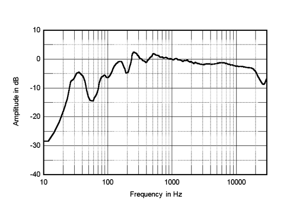
 The black trace below 300Hz in fig.3 shows the complex sum of the nearfield woofer and port responses, taking into account acoustic phase and the fact that the port is on the speaker's rear. The Vivid's low frequencies shelve down a little between 40Hz and 120Hz, and the usual boost in the upper bass due to the nearfield measurement technique is absent. As Vivid's Matt Longbottom implied in HR's review, the Kaya S12's low frequencies will benefit from the boundary reinforcement of placement relatively close to the front and side walls. The black trace above 300Hz in fig.3 shows the Kaya S12's farfield response averaged across a 30° horizontal window centered on the tweeter axis. Other than a very narrow spike at 5.8kHz, the speaker's response is extraordinarily flat throughout the midrange and treble. The output between 10kHz and 20kHz is 1–2dB too high in level, but the output drops above 20kHz due to the effect of the high-Q tweeter dome resonance at 30.6kHz.
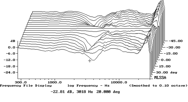
The Vivid's horizontal dispersion is shown in fig.4. (The traces are normalized to the response on the tweeter axis, which thus appears as a straight line.) Other than a slight lack of energy in the presence region to the sides, which might make the speaker sound a little polite, the contour lines in this graph are smooth and even, which correlates with accurate and stable stereo imaging. The Kaya S12 becomes a little more directional in the octave below 20kHz, which will tend to compensate for the slight excess of on-axis energy in this region. This graph also shows that the tweeter resonance is higher in level off-axis.
The black trace below 300Hz in fig.3 shows the complex sum of the nearfield woofer and port responses, taking into account acoustic phase and the fact that the port is on the speaker's rear. The Vivid's low frequencies shelve down a little between 40Hz and 120Hz, and the usual boost in the upper bass due to the nearfield measurement technique is absent. As Vivid's Matt Longbottom implied in HR's review, the Kaya S12's low frequencies will benefit from the boundary reinforcement of placement relatively close to the front and side walls. The black trace above 300Hz in fig.3 shows the Kaya S12's farfield response averaged across a 30° horizontal window centered on the tweeter axis. Other than a very narrow spike at 5.8kHz, the speaker's response is extraordinarily flat throughout the midrange and treble. The output between 10kHz and 20kHz is 1–2dB too high in level, but the output drops above 20kHz due to the effect of the high-Q tweeter dome resonance at 30.6kHz.
The Vivid's horizontal dispersion is shown in fig.4. (The traces are normalized to the response on the tweeter axis, which thus appears as a straight line.) Other than a slight lack of energy in the presence region to the sides, which might make the speaker sound a little polite, the contour lines in this graph are smooth and even, which correlates with accurate and stable stereo imaging. The Kaya S12 becomes a little more directional in the octave below 20kHz, which will tend to compensate for the slight excess of on-axis energy in this region. This graph also shows that the tweeter resonance is higher in level off-axis.
 The Vivid's vertical dispersion, again normalized to the response on the tweeter axis, is shown in fig.5. The Kaya S12's balance is maintained over a ±5° window centered on the tweeter axis, which is 34" from the floor with the speaker bolted to its dedicated stand. (A survey conducted for Stereophile by Thomas J. Norton in the 1990s indicated that 36" was the average ear height for seated listeners.) Above and below that window, however, a significant suckout in the crossover region makes an appearance.

Footnote 1: EPDR is the resistive load that gives rise to the same peak dissipation in an amplifier's output devices as the loudspeaker. See "Audio Power Amplifiers for Loudspeaker Loads," JAES, Vol.42 No.9, September 1994, and stereophile.com/reference/707heavy/index.html.
Fig.1 Vivid Kaya S12, electrical impedance (solid) and phase (dashed) (2 ohms/vertical div.).
The traces in fig.1 are free from the small discontinuities that would imply the presence of resonances of some kind. When I investigated the enclosure's vibrational behavior with a plastic-tape accelerometer, I found a couple of resonant modes on the curved sidewall, the highest in level lying at 199Hz (fig.2). However, this mode has a low amplitude and a moderately high Q (Quality Factor), both factors that will work against audibility. Fig.2 was taken with the Kaya S12's base bolted to the speaker's dedicated stand. I repeated the measurement with the speaker sitting on three upturned cones, these placed at the perimeter of its base. (This will be the worst case, as it allows resonant modes to develop fully.) I was surprised, therefore, to find that the resonant modes were now lower in both level and Q. However, the hashy-looking behavior between 1kHz and 2kHz in fig.2 was higher in level without the stand.
Fig.2 Vivid Kaya S12, cumulative spectral-decay plot calculated from output of accelerometer fastened to center of sidewall with speaker bolted to matching stand (MLS driving voltage to speaker, 7.55V; measurement bandwidth, 2kHz).
The saddle centered on 44Hz in the impedance-magnitude trace suggests that this is the tuning frequency of the rear-panel port that reflex-loads the woofer. The red trace in fig.3 shows the port's nearfield output. The response peaks sharply at 40Hz, and the upper-frequency rolloff is clean. The nearfield response of the woofer (fig.3, blue trace below 300Hz) has the expected notch at the port tuning frequency, which is when the back pressure from the port resonance holds the diaphragm stationary.
Fig.3 Vivid Kaya S12, anechoic response on tweeter axis at 50", averaged across 30° horizontal window and corrected for microphone response with the nearfield response of the port (red), woofer (blue), and their complex respectively plotted below 325Hz, 300Hz, and 300Hz.
Fig.4 Vivid Kaya S12, lateral response family at 50", normalized to response on tweeter axis, from back to front: differences in response 90–5° off axis, reference response, differences in response 5–90° off axis.
Fig.5 Vivid Kaya S12, vertical response family at 50", normalized to response on tweeter axis, from back to front: differences in response 45–5° above axis, reference response, differences in response 5–45° below axis.
After the review had been prepared for publication, I measured the Vivid S12's spatially averaged response in my own listening room (fig.6). I didn't have time to optimize the placement by moving the speakers closer to the sidewalls and the wall behind the speakers, which means the low-frequencies are shelved down. But note the superbly even response in the upper midrange and treble. Other than a slight excess of energy in the mid-treble region, the trace gently slopes down in the optimal manner as the frequency increases.
Fig.6 Vivid Kaya S12, spatially averaged, 1/6-octave response in JA's listening room.
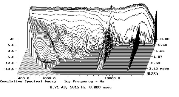
In the time domain, the Kaya S12's step response on the tweeter axis (fig.7) indicates that both drivers are connected in positive acoustic polarity and that the tweeter's output arrives first at the microphone. The decay of the tweeter's step blends smoothly with the start of the woofer's step, suggesting optimal crossover design. The Vivid's cumulative spectral-decay plot (fig.8) is impressively clean, with the exception of a narrow ridge of delayed energy at 5.8kHz, the frequency of that small spike in the fig.3 response. (As always, ignore the apparent ridge of low-level energy just below 16kHz in fig.8, which is due to interference from the MLSSA host computer's video circuitry.)
Fig.7 Vivid Kaya S12, step response on tweeter axis at 50" (5ms time window, 30kHz bandwidth).
Fig.8 Vivid Kaya S12, cumulative spectral-decay plot on tweeter axis at 50" (0.15ms risetime).
The Vivid Kaya S12's measured performance is indicative of the superb loudspeaker engineering I have come to expect from this brand.—John Atkinson
Footnote 1: EPDR is the resistive load that gives rise to the same peak dissipation in an amplifier's output devices as the loudspeaker. See "Audio Power Amplifiers for Loudspeaker Loads," JAES, Vol.42 No.9, September 1994, and stereophile.com/reference/707heavy/index.html.