Understanding Information Diagrams
 Sounds in the red-shaded area are probably inaudible. Components appearing in the grey and blue shaded areas contribute generally only by direct correlation with signals below 20kHz. With current state of the art, components above 48kHz exceed the playback capability of almost all loudspeakers and headphones.[28]
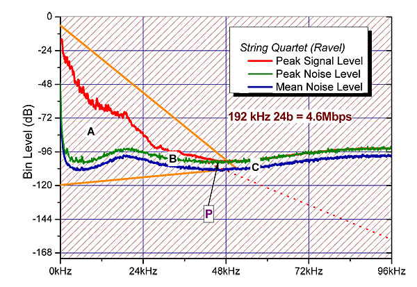 The peak level collected by the microphone shows a declining spectrum with increasing frequency. This is a very typical feature of naturally occurring sounds, one that can be exploited to reduce both temporal blur and data rate.
Note that the music and noise curves converge at 'P'—there are probably signal components above that frequency which are lost in the noise.
The region marked 'A' is in the conventional audio band—we are responsive to tones up to 20kHz. Region 'B' also contains music content, but none of that range is audible if heard in isolation; however elements in 'B' do contribute to the temporal resolution and sonic envelope but do not appear in isolation; experience shows that removing these lowers fidelity.
Region 'C' is different: it carries no salient music-dependent information, is above the passband of almost all microphones and loudspeakers and is also both below and beyond human thresholds for noise signals.
This steady noise is quite inaudible, however the higher sampling rate can enable improved resolution in region 'A,' the higher sample rate lowering blur.
As noted earlier, in acoustic recordings, point 'P' is observed between 30 and 60kHz, with 40kHz being typical. So, as sample rates are increased above 96kHz, for example to 192 or 352.8kHz, region 'C' extends over a wider bandwidth. In that region any music-correlated components are well below the noise, however there can be improved sound reproduction because the higher transmission rate enables less filter blur and better convergence.
So, the orange triangle in Figure 19 encloses all the musically relevant part of the signal (the remainder is noise and silence) and has an area of about one-sixth of the entire coding space—which means that five-sixths of the data rate is squandered.
The peak level collected by the microphone shows a declining spectrum with increasing frequency. This is a very typical feature of naturally occurring sounds, one that can be exploited to reduce both temporal blur and data rate.
Note that the music and noise curves converge at 'P'—there are probably signal components above that frequency which are lost in the noise.
The region marked 'A' is in the conventional audio band—we are responsive to tones up to 20kHz. Region 'B' also contains music content, but none of that range is audible if heard in isolation; however elements in 'B' do contribute to the temporal resolution and sonic envelope but do not appear in isolation; experience shows that removing these lowers fidelity.
Region 'C' is different: it carries no salient music-dependent information, is above the passband of almost all microphones and loudspeakers and is also both below and beyond human thresholds for noise signals.
This steady noise is quite inaudible, however the higher sampling rate can enable improved resolution in region 'A,' the higher sample rate lowering blur.
As noted earlier, in acoustic recordings, point 'P' is observed between 30 and 60kHz, with 40kHz being typical. So, as sample rates are increased above 96kHz, for example to 192 or 352.8kHz, region 'C' extends over a wider bandwidth. In that region any music-correlated components are well below the noise, however there can be improved sound reproduction because the higher transmission rate enables less filter blur and better convergence.
So, the orange triangle in Figure 19 encloses all the musically relevant part of the signal (the remainder is noise and silence) and has an area of about one-sixth of the entire coding space—which means that five-sixths of the data rate is squandered.
 A 16-bit/44.1kHz digital file can be delivered losslessly but that doesn't ensure that it achieves blameless end-to-end sound quality, far from it.
The same is true of conventional hi-rez digital because, while potentially superior to 16-bit/44.1kHz, it has not been specified to match the time-domain acuity of human hearing.
So the goal of MQA is not lossless operation in this narrow, technical sense, even though its core digital path is lossless and bit-for-bit determined and confirmed by the decoder. The goal is to capture and deliver everything we can hear, without the inherent blur of conventional sampling, without the uncertainty of converter quantizations, and to convey the analogue sound heard in the mastering studio to the end-user without modification. This makes it 'lossless' in a much more profound, and relevant, way. [13]
A 16-bit/44.1kHz digital file can be delivered losslessly but that doesn't ensure that it achieves blameless end-to-end sound quality, far from it.
The same is true of conventional hi-rez digital because, while potentially superior to 16-bit/44.1kHz, it has not been specified to match the time-domain acuity of human hearing.
So the goal of MQA is not lossless operation in this narrow, technical sense, even though its core digital path is lossless and bit-for-bit determined and confirmed by the decoder. The goal is to capture and deliver everything we can hear, without the inherent blur of conventional sampling, without the uncertainty of converter quantizations, and to convey the analogue sound heard in the mastering studio to the end-user without modification. This makes it 'lossless' in a much more profound, and relevant, way. [13]
Footnote 6: The microphone limit can be thought of as 'absolute zero' for recordings on earth, signals below this are random noise and we don't need to preserve them precisely.
Figure 18: Shannon diagram showing the capacity of digital channels (area is equivalent to data rate).
Figure 18 compares the coding space for a number of common transmission formats, including CD, and 96 and 192kHz at 24- and 32-bit depths; also shown is the noise-floor for DSD64.
To accommodate the coding capacity of 32-bit LPCM, the vertical scale of this graph is formidable. At the top, 120dB SPL is the threshold of pain; 0dB (the quietest we can perceive) is in the center. The noise-floor of the 32-bit channel is 120dB lower than silence, so although more bits give us a finer staircase, the channel's information capacity is excessive.
Four additional curves provide perspective: red is the noise-spectral human threshold (wideband noise below this line is not heard directly); green, typical quiet out-door environmental sound; navy, the noise-floor of the quietest commercial recording in our survey and, finally, brown, the fundamental thermal noise limit for a microphone (data below this line are Brownian motion, footnote 6). [6]
Figure 19: Shannon diagram of an example 24-bit/192kHz recording showing signal and noise levels.
Figure 19 is a Shannon diagram showing the entire coding space for a 24-bit/192kHz source signal and, within it, in red, the peak frequency spectrum of real audio—in this case a movement from a Ravel string quartet. The green and blue curves, respectively, show the peak and mean of the recording's background noise—that is the sound we hear before, during and after the music—that is comprised of hall ambience and some analogue noise.
This recording was chosen as a worked example because it is of real instruments in a natural acoustic. The plucked pizzicato strings are challenging to reproduce and the spectrum shows harmonic components well above 20kHz, which contribute to the sonic envelope.
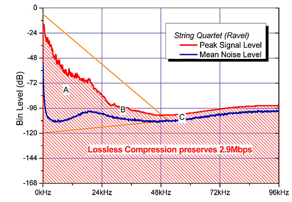
Figure 20: Application of MLP lossless compression reduces the data rate from 4.6 to 2.9 Mbps.
High-performance lossless compression can improve matters by reducing the data rate to 2.9 Mbps per channel, a saving of 37%, but this is still inefficient and too high to be ideal for streaming from online music services.
The goal of MQA is to deliver the contents of the orange triangle precisely, with increased and extreme precision, while avoiding temporal blur or noise modulation in the converters. To achieve this MQA goes 'beyond lossless' in the sense that it has at its core a realisation that 'lossless', as the term is usually used, is no guarantor of ultimate sound quality because it does not embrace the A/D and D/A conversion, volume control etc.
Footnote 6: The microphone limit can be thought of as 'absolute zero' for recordings on earth, signals below this are random noise and we don't need to preserve them precisely.