Sidebar 3: Measurements
Because of the Wilson Sasha DAW's bulk and weight—as well as the fact that Sasha Matson's listening room is on the second floor of his upstate New York home—I drove my test gear the 230 miles from my Brooklyn home to measure the speakers in situ. (I also wanted to hear the Wilson speakers driven by his McIntosh MC462 amplifier, which had impressed me when I measured it for our May 2019 issue.)
As always, I used DRA Labs' MLSSA system and a calibrated DPA 4006 microphone to measure the Sasha DAW's frequency response in the farfield and an Earthworks QTC-40 mike for the nearfield responses. When testing a loudspeaker, I raise it off the floor so that the tweeter is midway between the ceiling and floor. This maximizes the anechoic time window, hence the midrange resolution, of the FFT-based response measurements. Sasha M and I managed to lift one of the 236lb Sasha DAWs onto a small dolly, to make it easier to move it as necessary, but the inevitable reflection of the speaker's sound from the floor reduces the accuracy of my measurements in the midrange.
With that caution in mind, Wilson specifies the Sasha DAW's sensitivity as 91dB/W/1m. My estimate was slightly lower, at 89.5dB(B)/2.83V/m, but this is still usefully higher than average. The nominal impedance is 4 ohms with a minimum value of 2.48 ohms at 85Hz. My measurements of the Wilson's impedance magnitude (solid trace) and electrical phase angle (dotted trace) are shown in fig.1. While the impedance remains above 4 ohms above 160Hz, it drops to 2.415 ohms at 84Hz. The electrical phase angle (dashed trace) reaches –41.3° at 57Hz and +25.7° at 34Hz, both frequencies where the magnitude at 4.75 ohms and 5 ohms is relatively low. The Sasha DAW is an easier load than the Sasha W/P, which Art Dudley reviewed in July 2010, but its impedance will still be a challenge for the partnering amplifier. (This would not have been a problem for SM's McIntosh, however.)
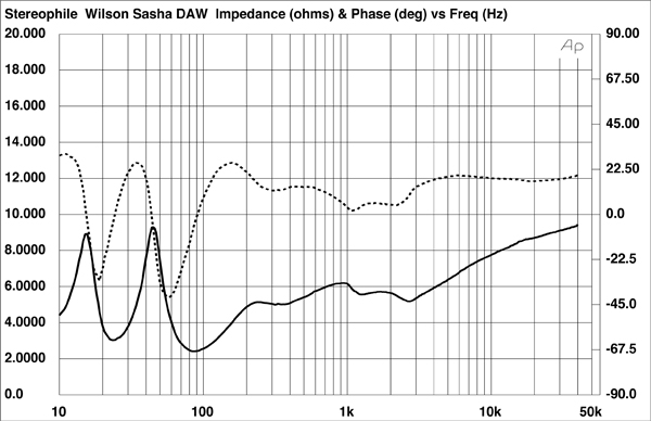
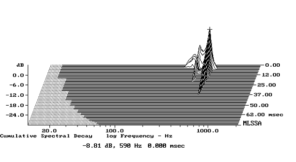
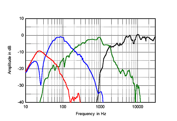
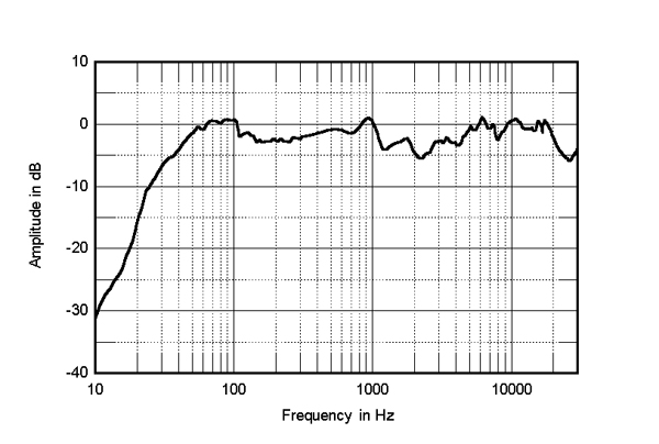
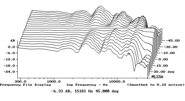
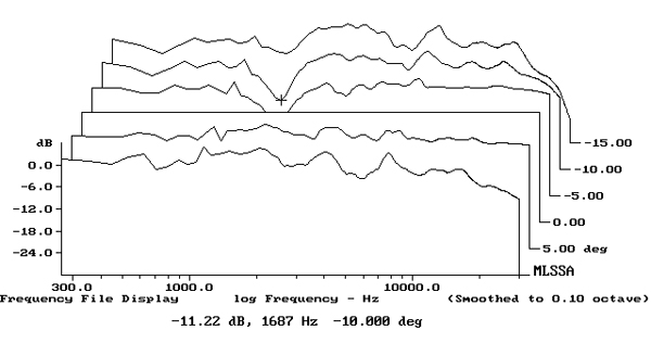
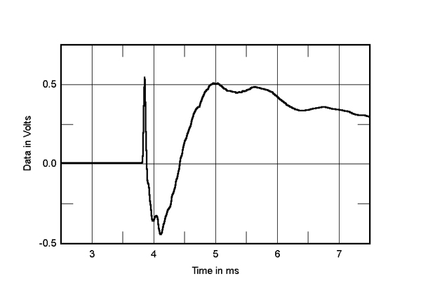
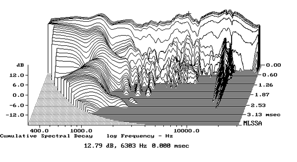
Fig.1 Wilson Sasha DAW, electrical impedance (solid) and phase (dashed) (2 ohms/vertical div.).
The impedance traces are free from the small discontinuities that would suggest the presence of panel resonances. The woofer bin was impressively inert, but when I investigated the upper enclosure's vibrational behavior with a plastic-tape accelerometer, I found a high-Q mode at 598Hz at two places on the sidewalls (fig.2). The high Q, the high frequency, and the fact that the affected areas are small all work against there being any audible problems resulting from the presence of this mode.
Fig.2 Wilson Sasha DAW, cumulative spectral-decay plot calculated from output of accelerometer fastened to upper-frequency enclosure sidewall close to the baffle (MLS driving voltage to speaker, 7.55V; measurement bandwidth, 2kHz).
The impedance-magnitude plot has a saddle centered on a low 23Hz, which will be due to the tuning frequency of the large port on the woofer cabinet's rear panel. The two woofers behave identically; the blue trace in fig.3 shows their summed nearfield response, which has its minimum-motion notch at the expected 23Hz. The nearfield response of the port (red trace) peaks at the same frequency and its upper-frequency rolloff is very clean. The woofers cross over to the midrange unit (green trace) around 200Hz with the rollout above that frequency free from any peaks. As with the earlier Sasha, the midrange unit's initial rolloff starts at 400Hz and is very gentle. The port on the rear of the upper enclosure is used to increase the midrange unit's power handling rather than to extend its low-frequency response with a traditional reflex alignment.
Fig.3 Wilson Sasha DAW, acoustic crossover on tweeter axis at 50", corrected for microphone response, with nearfield midrange (green), woofer (blue) and port (red) responses respectively plotted below 500Hz, 350Hz, and 300Hz.
Like other Wilson loudspeakers, the Sasha DAW's upper enclosure is mounted on the woofer bin with spikes and a series of steps at the rear to allow the midrange and tweeter to be aimed at the listener's ears. For the farfield response measurements in fig.3 and the following graphs, I calculated where the microphone should be placed on the tweeter axis at my standard 50" distance. The midrange unit's output on this axis has a slight peak at 1kHz before crossing over to the tweeter (black trace) just below 2kHz and rolling out relatively smoothly. Small peaks in the tweeter's output are balanced by small dips; the overall response trend is even.
The Wilson's farfield response, averaged across a 30° horizontal window centered on the tweeter axis, is shown as the black trace above 300Hz in fig.4. The overall balance is even from the upper bass through to the top of the audioband, though there is a lack of presence-region energy. The black trace below 300Hz in fig.4 shows the sum of the nearfield woofer and port outputs, taking into account acoustic phase and the different distance of each radiator from a nominal farfield microphone position. The usual rise in response in the upper bass that is due to the nearfield measurement technique is absent. I suspect that the Wilson's low-frequency alignment is optimized for definition rather than maximum bass power. With the low tuning frequency of the port, boundary reinforcement will give extension to 20Hz with typical low-frequency room gain. Certainly in my own auditioning of the Sasha DAWs in Sasha M's relatively small room, the bass sounded both full-range and powerful, but with superb leading-edge clarity.
Fig.4 Wilson Sasha DAW, anechoic response on tweeter axis at 50", averaged across 30° horizontal window and corrected for microphone response, with the complex sum of the nearfield midrange, woofer, and port responses plotted below 300Hz.
The Wilson Sasha DAW's horizontal dispersion, normalized to the tweeter- axis response, is shown in fig.5. (Due to the geometric limitations of SM's room, I could only plot the differences in response up to 45° each side of the tweeter axis instead of my usual 90°.) This graph indicates that some of the missing presence-region energy reap- pears to the speaker's sides. The contour lines in this graph are otherwise even, implying stable stereo imaging. In the vertical plane (fig.6), a suckout develops in the crossover region 5° above the tweeter axis. However, there is more energy present between 1kHz and 3kHz 5° below the measurement axis, which suggests I should have placed the microphone a little lower to be on the exact axis intended by Peter McGrath when he set the speakers up in SM's room.
Fig.5 Wilson Sasha DAW, lateral response family at 50", normalized to response on tweeter axis, from back to front: differences in response 45–5° off axis, reference response, differences in response 5–45° off axis.
Fig.6 Wilson Sasha DAW, vertical response family at 50", normalized to response on tweeter axis, from back to front: differences in response 15–5° above axis, reference response, differences in response 5–10° below axis.
This conjecture is confirmed by the Sasha DAW's step response (fig.7), which is almost identical to that of the Wilson Alexia 2 that I reviewed in July 2018. The tweeter's positive-going step arrives first at the microphone but has started to decay before the start of the midrange unit's negative-going step. The optimal blend between the two units' steps occurs a little lower than the axis that I had calculated I should use for the farfield measurements. However, the positive-going decay of the midrange step does blend smoothly with the start of the woofer's step, which indicates an optimal crossover topology. The Wilson's cumulative spectral-decay plot (fig.8) is relatively clean overall, though some low-level delayed energy is present in the treble. There is also some delayed energy associated with the small on-axis peak at 1kHz.
Fig.7 Wilson Sasha DAW, step response on tweeter axis at 50" (5ms time window, 30kHz bandwidth).
Fig.8 Wilson Sasha DAW, cumulative spectral-decay plot on tweeter axis at 50" (0.15ms risetime).
The Sasha DAW's measured performance has much in common with the other Wilson speakers I have measured and indicates a careful balance between frequency and time domains.—John Atkinson