Sidebar 3: Measurements
I used DRA Labs' MLSSA system and a calibrated DPA 4006 microphone to measure the Magico M2's frequency response in the farfield, and an Earthworks QTC-40 mike for the nearfield and in-room responses. The 165lb loudspeaker was too bulky to move outside for testing or to lift onto my computer-controlled turntable. I therefore had to do the quasi-anechoic measurements in my listening room, where the proximity of room boundaries led to more aggressive windowing of the time-domain data than usual, which in turn reduced the graphs' resolution in the midrange.
Although Magico specifies the M2's sensitivity as 88dB/W/m, my estimate was slightly lower, at 86dB(B)/2.83V/m. The M2's impedance is specified as 4 ohms. My measurements indicated that the impedance magnitude (fig.1, solid trace) was close to 4 ohms in the midrange but drops to 2.3 ohms between 74Hz and 88Hz. The electrical phase angle (dashed trace) reaches –71° at 50Hz. Although the magnitude at this frequency is 6.5 ohms, this phase angle significantly increases the current needed from the amplifier. This, and the combination of 3.2 ohms and –54.5° at 60Hz, means the M2 will be a demanding load. The single impedance peak at 40Hz indicates that this is the tuning frequency of the M2's woofers. The reduction in impedance above the audioband, in combination with an increasingly negative phase angle, is unusual. Loudspeakers typically have a rising magnitude in this region coupled with an increasingly positive phase angle, these both due to the tweeter's voice-coil inductance.
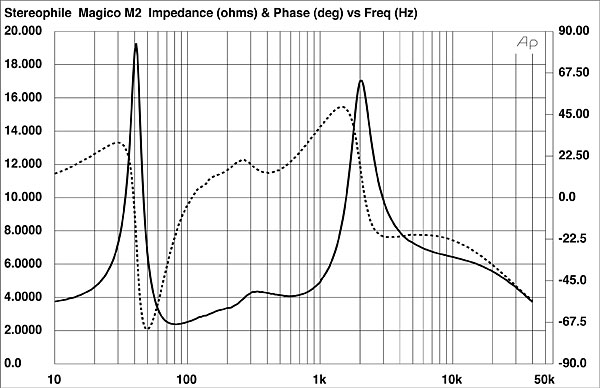
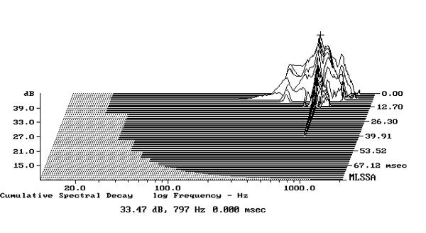
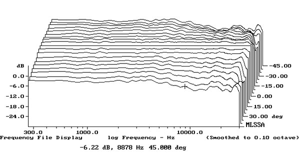
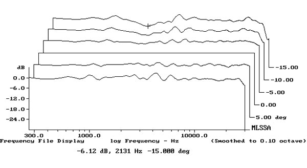
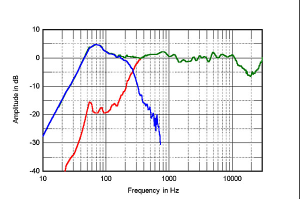 Fig.4 shows the Magico's horizontal dispersion, referenced to the response on the tweeter axis, which thus appears as a straight line. The contour lines in this graph are evenly spaced throughout the midrange and treble, implying stable stereo imaging, and, commendably, the M2's on-axis balance in the treble is maintained to >30° to the sides. In the vertical plane (fig.5), a suckout starts to develop in the crossover region 15° above the tweeter axis. Even so, the M2 maintains its tweeter-axis balance over a wide ±10° vertical window.
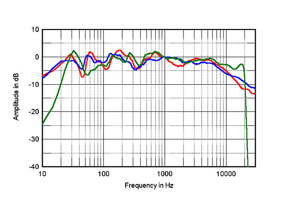
 The red trace in fig.6 shows the M2s' spatially averaged response in my room. This is generated by averaging 20 1/6-octave–smoothed spectra, taken for the left and right speakers individually using a 96kHz sample rate, in a vertical rectangular grid 36" wide by 18" high and centered on the positions of my ears. For reference, the blue trace shows the spatially averaged response of the Magico S5 Mk.II that I reviewed in February 2017, while the green trace is the spatially averaged response of the Q Acoustics Concept 300 I reviewed in the January 2020 issue. (Because the Q Acoustics' response was taken with the NAD M10 amplifier, which digitizes its analog inputs at 44.kHz, the green trace drops like a stone above 20kHz.)
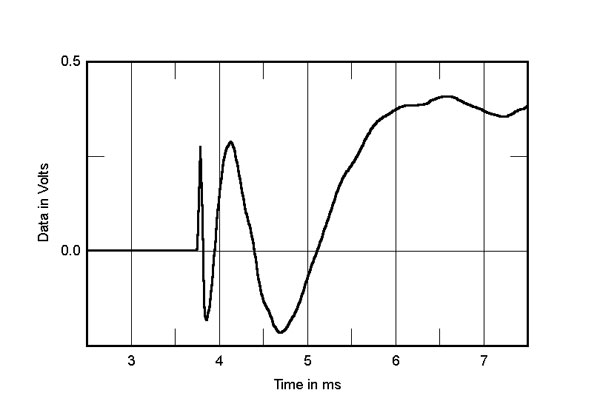
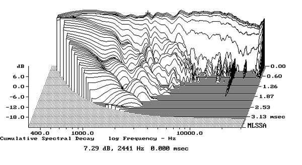
 In the time domain, the M2's step response (fig.7) indicates that all four drive-units are connected in positive acoustic polarity. The decay of the tweeter's step, which arrives first at the microphone, smoothly blends with the start of the midrange unit's step, the decay of which blends smoothly with the start of the woofers' step. This time-coherent behavior suggests optimal crossover implementation. The Magico M2's cumulative spectral-decay plot (fig.8) is superbly clean overall, though with some low-level delayed energy apparent at the top of the midrange unit's passband.
Footnote 1: This graph was not taken with MLSSA so the Y-axis level is not calibrated. It cannot be compared with cabinet vibrational cumulative spectral-decay plots in other Stereophile loudspeaker reviews.
Fig.1 Magico M2, electrical impedance (solid) and phase (dashed) (2 ohms/vertical div.).
The traces in fig.1 are free from the small discontinuities that would imply resonances. When I investigated the enclosure's vibrational behavior with a plastic-tape accelerometer, with the speaker sitting on its MPod stands, I found that there was a low-level mode at 797Hz on the sidewalls (footnote 1). The relatively high frequency and Q (Quality Factor) make it unlikely that this mode will have any audible consequences.
Fig.2 Magico M2, cumulative spectral-decay plot calculated from output of accelerometer fastened to center of sidewall level with midrange unit (MLS driving voltage to speaker, 4V; measurement bandwidth, 2kHz).
The blue trace in fig.3 shows the woofers' summed nearfield response. (Both woofers behaved identically.) The slight peak in the bass is almost entirely due to the nearfield measurement technique, which assumes that the drive-unit is firing into half-space rather than in all directions. The woofers cross over to the midrange unit (red trace) just below 300Hz, with a fast rolloff that is peak-free. The Magico's farfield response, averaged across a 30° horizontal window centered on the tweeter axis, is shown as the green trace above 300Hz in fig.3. The balance is superbly flat and even, though with a slight excess of energy in the upper midrange. Unusually, the M2's output in the top audio octave slopes gently down before starting to rise again above 20kHz. I repeated this measurement with the Dayton OmniMic system as well as with FuzzMeasure using the Earthworks QTC-40 microphone. While the OmniMic system is limited to 20kHz, the Earthworks has a 40kHz bandwidth. The FuzzMeasure measurement with the QTC-40 confirmed that the M2's response rises again above 20kHz, with a small peak present at 22.5kHz and a higher-level peak close to 35kHz. I understand that with a tweeter using a pistonic hard dome with a high-Q, high-amplitude, ultrasonic resonance, there will be a lack of energy in the region below that resonance.
Fig.3 Magico M2, anechoic response on tweeter axis at 50", averaged across 30° horizontal window and corrected for microphone response (green), with the nearfield responses of the midrange unit (red) and woofers (blue) respectively plotted below 350Hz and 7 00Hz.
Fig.4 Magico M2, lateral response family at 50", normalized to response on tweeter axis, from back to front: differences in response 45–5° off axis, reference response, differences in response 5–45° off axis.
Fig.5 Magico M2, vertical response family at 50", normalized to response on tweeter axis, from back to front: differences in response 15–5° above axis, reference response, differences in response 5–10° below axis.
Fig.6 Magico M2, spatially averaged, 1/6-octave response in JA's listening room (red), of the Magico S5 Mk.II (blue), and of the Q Acoustics Concept 300 (green).
While performing these measurements, I noticed that the responses at the listening position of the two M2s matched very closely above 900Hz. The in-room response of the two Magico designs is very similar in the bass and midrange, though the M2 and the Concept 300 have slightly greater output between 600Hz and 1kHz than the S5 Mk.II has. The M2 has less energy between 1kHz and 2kHz than the other two speakers have, though all three behave similarly in the low to mid-treble. The slightly sloped-down output above 7kHz of both Magico speakers is due to the increased absorptivity of the room's furnishings at higher frequency, though the M2 produces less energy above 13kHz in-room than the S5 Mk.II. By contrast, the Q Acoustics speaker has significantly more top-octave output than the two pairs of Magicos have.
Fig.7 Magico M2, step response on tweeter axis at 50" (5ms time window, 30kHz bandwidth).
Fig.8 Magico M2, cumulative spectral-decay plot on tweeter axis at 50" (0.15ms risetime).
As with the other Magico loudspeakers Stereophile has reviewed, the M2 offers excellent measured performance.—John Atkinson
Footnote 1: This graph was not taken with MLSSA so the Y-axis level is not calibrated. It cannot be compared with cabinet vibrational cumulative spectral-decay plots in other Stereophile loudspeaker reviews.